arc3d · area · define_shape · diam · diam3d · diam_changed · distance · getSpineArea · L · n3d · pt3dadd · pt3dchange · pt3dclear · pt3dconst · pt3dinsert · pt3dremove · pt3dstyle · Ra · ri · setSpineArea · spine3d · x3d · y3d · z3d

Conceptual Overview of Sections

Sections are unbranched lengths of continuous cable connected together to form a neuron. Sections can be connected to form any tree-shaped structure but loops are not permitted. (You may, however, develop membrane mechanisms, such as electrical gap junctions which do not have the loop restriction. But be aware that the electrical current flows through such connections are calculated by a modified euler method instead of the more numerically robust fully implicit/crank-nicholson methods)

Do not confuse sections with segments. Sections are divided into segments of equal length for numerical simulation purposes (see Section.nseg). NEURON uses segments to represent the electrical circuit shown below.

          Ra
o/`--o--'\/\/`--o--'\/\/`--o--'\/\/`--o--'\o v
     |          |          |          |
    ---        ---        ---        ---
   |   |      |   |      |   |      |   |
    ---        ---        ---        ---
     |          |          |          |
-------------------------------------------- ground

Such segments are similar to compartments in compartmental modeling programs.

Geometry

Section geometry is used to compute the area and axial resistance of each segment.

There are two ways to specify section geometry:

The stylized method simply specifies parameters for length and diameter.
The 3-D method specifies a section’s shape, orientation, and location in three dimensions.

Choose the stylized method if the notions of cable length and diameter are authoritative and where 3-d shape is irrelevant. For plotting purposes, length and diameter will be used to generate 3-d info automatically for a stylized straight cylinder. (see define_shape())

Choose the 3-D method if the shape comes from 3-d reconstruction data or if your 3-d visualization is paramount. This method makes the 3-d info authoritative and automatically determines the abstract cable’s length and diameter. With this method, you may change a section’s length/diameter only by changing it’s 3-d info. (but see pt3dconst())

Stylized specification of geometry

For simulations one needs to specify L, nseg, diam, Ra, and connectivity.

section.L: For each section, L is the length of the entire section in microns.
section.nseg: The section is divided into nseg compartments of length L/nseg. Membrane potential will be computed at the ends of the section and the middle of each compartment.
seg.diam: The diameter in microns. Note that diam is a range variable and therefore must be respecified whenever nseg is changed.
section.Ra: Axial resistivity in ohm-cm.
connectivity: This is established with the connect command and defines the parent of the section, which end of the section is attached to the parent, and where on the parent the attachment takes place. To avoid confusion, it is best to attach the 0 end of a section to the 1 end of its parent.

In the stylized specification, the shape model used for a section is a sequence of right circular cylinders of length, L/nseg, with diameter given by the diam range variable at the center of each segment. The area of a segment is PI*diam*L/nseg (micron2) and the half-segment axial resistance is .01*sec.Ra*(L/2/sec.nseg)/(PI*(seg.diam/2)^2). The .01 factor is necessary to convert ohm-cm micron/micron2 to MegOhms. Ends of cylinders are not counted in the area and, in fact, the areas are very close to those of truncated cones as long as the diameter does not change too much.

from neuron import h
import numpy

sec = h.Section(name='sec')
sec.nseg = 11
sec.Ra = 100
sec.L = 1000
# linearly interpolate diameters from 11 to 100
for seg in sec:
    seg.diam = numpy.interp(seg.x, [0, 1], [11, 100])

for seg in sec.allseg():
    print(seg.x, seg.diam, seg.area(),
          h.PI * seg.diam * sec.L / sec.nseg, seg.ri(),
          0.01 * sec.Ra * sec.L / 2 / sec.nseg / (h.PI * (seg.diam / 2) ** 2))

Output:

0 14.5 0.0 4555.309347705201 1e+30 0.30279180612013384
05 14.5 4555.3093477052 4555.309347705201 0.30279180612013384 0.30279180612013384
15 23.5 7382.7427359360145 7382.742735936014 0.41806926603277866 0.11527745991264488
25 32.5 10210.176124166826 10210.176124166826 0.17554915433797802 0.060271694425333144
35 41.5 13037.609512397643 13037.609512397643 0.09723611726566303 0.03696442284032988
45 50.5 15865.042900628456 15865.042900628458 0.061927456753380815 0.024963033913050933
55 59.50000000000001 18692.47628885927 18692.47628885927 0.04294537336273899 0.01798233944968805
65 68.5 21519.909677090083 21519.909677090083 0.0315498128871132 0.013567473437425146
75 77.5 24347.343065320896 24347.343065320896 0.02416676205124544 0.010599288613820293
85 86.5 27174.77645355171 27174.77645355171 0.019107688792477533 0.00850840017865724
95 95.5 30002.209841782525 30002.209841782525 0.015488688793197206 0.006980288614539967
0 95.5 0.0 30002.209841782525 0.006980288614539967 0.006980288614539967

Note that the area (and length) of the 0,1 terminal ends is equal to 0 and the axial resistance is the sum of the adjacent half-segment resistances between segment and parent segment. Such, niceties allow the spatial discretization error to be proportional to (1/nseg)^2. However, for second order correctness, all point processes must be located at the center of the segments or at the ends and all branches should be connected at the ends or centers of segments. Note that if one increases nseg by a factor of 3, old centers are preserved.

For single compartment simulations it is most convenient to choose a membrane area of 100 micron² so that point process currents (nanoamps) are equivalent to density currents (milliamps/cm²).

Also note that a single compartment of length = diameter has the same effective area as that of a sphere of the same diameter.

Example:

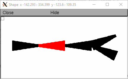
The following example demonstrates the automatic 3-d shape construction. The root section “a” is drawn with it’s 0 end (left) at the origin and is colored red.

Sections connected to its 1 end (sections b, c, d) get drawn from left to right. Sections descended from the 0 end (section e) of the root get drawn from right to left.

Especially note the diameter pattern of section c whose “1” end is connected to the “b” parent. You don’t have to understand this if you always connect the “0” end to the parent.

from neuron import h, gui
import numpy

a, b, c, d, e = [h.Section(name=n) for n in ['a', 'b', 'c', 'd', 'e']]
b.connect(a)
c.connect(b(1), 1) # connect the 1 end of c to the 1 end of b
d.connect(b)
e.connect(a(0)) # connect the 0 end of e to the 0 end of a
for sec in h.allsec():
    sec.nseg = 21
    sec.L = 100
    for seg in sec:
        seg.diam = numpy.interp(seg.x, [0, 1], [10, 40])

s = h.Shape()
s.show(False)
s.color(2, sec=a) # color section "a" red
h.topology()
h.finitialize(-65)
for sec in h.allsec():
    print(sec)
    for i in range(sec.n3d()):
        print(f'{i}: ({sec.x3d(i)}, {sec.y3d(i)}, {sec.z3d(i)}; {sec.diam3d(i)})')

If you change the diameter or length, the Shape instances are automatically redrawn or when doNotify() is called. Segment area and axial resistance will be automatically recomputed prior to their use.

Under some circumstances, involving nonlinearly varying diameters across a section, at first sight surprising results can occur when the stylized method is used and a Shape instance is created. This is because under a define_shape() with no pre-existing 3-d points in a section, a number of 3-d points is created equal to the number of segments plus the end areas. When 3-d points exist, they determine the calculation of L, diam, area, and ri. Thus diam can change slightly merely due to shape creation. When L and diam are changed, there is first a change to the 3-d points and then L and diam are updated to reflect the actual values of these 3-d points. Due to multiple interpolation effects, specifying a nonlinearly varying diam will, in general, not give exactly the same diameter values as the case where no 3-d information exists. This effect is illustrated in the following example

from neuron import h, gui

def pr(nseg):
    sec.pt3dclear()
    sec.nseg = nseg
    setup_diam()
    h.define_shape()
    print_stats()

def setup_diam():
    for seg in sec:
        seg.diam = 20 if 0.34 <= seg.x <= 0.66 else 10

def print_stats():
    for seg in sec.allseg():
        print(seg.x * sec.L, seg.diam, seg.area(), seg.ri())

h.xpanel("change nseg")
h.xradiobutton("nseg = 3", (pr, 3))
h.xradiobutton("nseg = 11", (pr, 11))
h.xradiobutton("nseg = 101", (pr, 101))
h.xpanel()

sec = h.Section(name='sec')
sec.Ra = 100
sec.L = 100
sec.nseg = 3
setup_diam()
print_stats()

s = h.Shape()
s.show(False)

for i in range(sec.n3d()):
    print(f'{i}: {sec.arc3d(i)} {sec.diam3d(i)}')

print(f"L= {sec.L}")
print_stats()

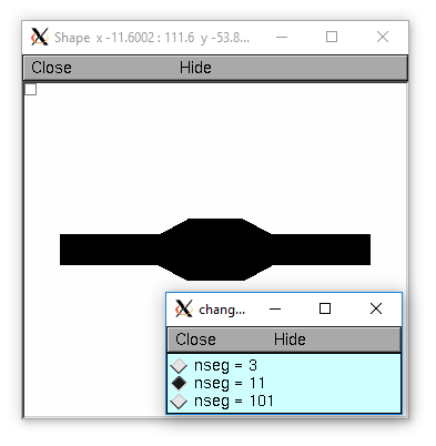
The difference is that the 3-d points define a series of truncated cones instead of a series of right circular cylinders. The difference is reduced with larger nseg. With the stylized method, abrupt changes in diameter should only take place at the boundaries of sections if you wish to view shape and also make use of the fewest possible number of segments. But remember, end area of the abrupt changes is not calculated. For that, you need an explicit pair of 3-d points with the same location and different diameters.

3-D specification of geometry

3-d information for a section is kept in a list of (x,y,z,diam) “points”. The first point is associated with the end of the section that is connected to the parent (NB: Not necessarily the 0 end) and the last point is associated with the opposite end. There must be at least two points and they should be ordered in terms of monotonically increasing arc length.

The root section is treated as the origin of the cell with respect to 3-d position. When any section’s 3-d shape or length changes, all the sections in the child trees have their 3-d information translated to correspond to the new position. So, assuming the soma is the root section, to translate an entire cell to another location it suffices to change only the location of the soma. It will avoid confusion if, except for good reason, one attaches only the 0 end of a child section to a parent. This will ensure that the sec(x).diam as x ranges from 0 to 1 has the same sense as sec.diam3d(i) as i ranges from 0 to sec.n3d()-1.

The shape model used for a section when the pt3d list is non-empty is that of a sequence of truncated cones in which the pt3d points define the location and diameter of the ends. From this sequence of points, the effective area, diameter, and resistance is computed for each segment via a trapezoidal integration across the segment length. This takes into account the extra area due to sqrt(dx^2 + dy^2) for fast changing diameters (even degenerate cones of 0 length can be specified, ie. two points with same coordinates but different diameters) but no attempt is made to deal with centroid curvature effects on the area. Note that the number of 3d points used to describe a shape has nothing to do with nseg and does not affect simulation speed. (Although, of course, it does affect how fast one can draw the shape)

Example:

The following illustrates the notion of the 3-d points as describing a sequence of cones. Note that the segment area and resistance is different than the simplistic calculation used in the stylized method. In this case the area of the segment has very little to do with the diameter of the center of the segment.

from neuron import h, gui
from math import sin, cos

sec = h.Section(name='sec')
sec.Ra=100
sec.nseg = 11
sec.pt3dclear()
for i in range(31):
    x = h.PI * i / 30.
    sec.pt3dadd(200 * sin(x), 200 * cos(x), 0, 100 * sin(4 * x))

s = h.Shape()
s.show(0)
print(sec.L)
for seg in sec.allseg():
    print(
        seg.x, seg.diam, seg.area(), h.PI * seg.diam * sec.L / sec.nseg,
        seg.ri(),
        0.01 * sec.Ra * sec.L / 2 / sec.nseg / (h.PI * (seg.diam / 2) ** 2))

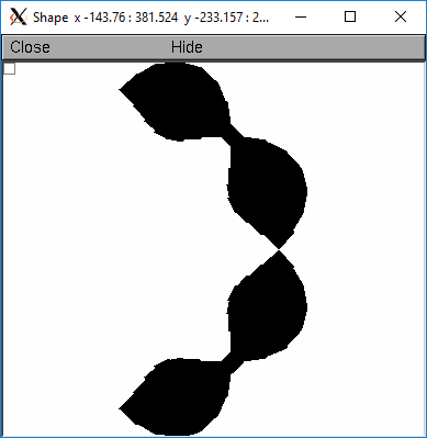
Note that at one point the diameter is numerically 0 and the axial resistance becomes essentially infinite thus decoupling the adjacent segments. Take care to avoid constructing spheres with a beginning and ending diameter of 0. No current would flow from the end to a connecting section. The end diameter should be the diameter of the end of the connecting section.

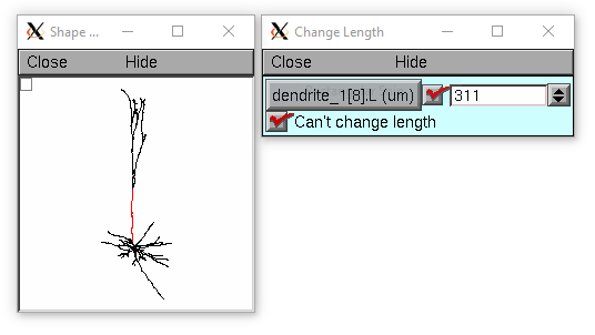
The following loads the pyramidal cell 3-d reconstruction from the demo directory of your neuron system. Notice that you can modify the length only if the pt3dconst mode is 0.

from neuron import h, gui
import __main__

h.xopen("$(NEURONHOME)/demo/pyramid.nrn")
mode = 1
h.pt3dconst(mode) # uses default section from pyramid.nrn
s = h.Shape()
s.action(lambda: s.select(sec=h.dendrite_1[8]))
s.color(2, sec=h.dendrite_1[8])

h.xpanel("Change Length")
h.xvalue("dendrite_1[8].L", "dendrite_1[8].L", 1) # using HOC syntax
                                                  # to directly access
                                                  # the length
h.xcheckbox("Can't change length", (__main__, 'mode'),
            lambda: h.pt3dconst(mode, sec=h.dendrite_1[8]))
h.xpanel()

See also

define_shape(), pt3dconst()

If 3-D shape is not an issue it is sufficient to specify the section variables L (length in microns), Ra (axial resistivity in ohm-cm), and the range variable diam (diameter in microns).

A list of 3-D points with corresponding diameters describes the geometry of a given section.

Defining the 3D Shape

pt3dclear()

Syntax:

buffersize = h.pt3dclear(sec=section)

buffersize = h.pt3dclear(buffersize, sec=section)

Description:

Destroy the 3d location info in section. With an argument, that amount of space is allocated for storage of 3-d points in that section.

Note

A more object-oriented approach is to use sec.pt3dclear() instead.

pt3dadd()

Syntax:

h.pt3dadd(x, y, z, d, sec=section)

h.pt3dadd(xvec, yvec, zvec, dvec, sec=section)

Description:

Add the 3d location and diameter point (or points in the second form) at the end of the current pt3d list. Assume that successive additions increase the arc length monotonically. When pt3d points exist in section they are used to compute diam and L. When diam or L are changed and h.pt3dconst(sec=section)==0 the 3-d info is changed to be consistent with the new values of L and diam. (Note: When L is changed, h.define_shape() should be executed to adjust the 3-d info so that branches appear connected.) The existence of a spine at this point is signaled by a negative value for d.

The vectorized form is more efficient than looping over lists in Python.

Example of vectorized specification:

from neuron import h, gui
import numpy

# compute vectors defining a geometry
theta = numpy.linspace(0, 6.28, 63)
xvec = h.Vector(4 * numpy.cos(theta))
yvec = h.Vector(4 * numpy.sin(theta))
zvec = h.Vector(theta)
dvec = h.Vector([1] * len(theta))

dend = h.Section(name='dend')
h.pt3dadd(xvec, yvec, zvec, dvec, sec=dend)

s = h.Shape()
s.show(0)

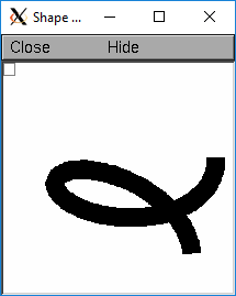
Note

The vectorized form was added in NEURON 7.5.

Note

A more object-oriented approach is to use sec.pt3dadd instead.

pt3dconst()

Syntax:

h.pt3dconst(0, sec=section)

h.pt3dconst(1, sec=section)

Description:

If pt3dconst is set at 0, newly assigned values for d and L will automatically update pre-existing 3d information. pt3dconst returns its previous state on each call. Its original value is 0.

Note that the diam information transferred to the 3d point information comes from the current diameter of the segments and does not change the number of 3d points. Thus if there are a lot of 3d points the shape will appear as a string of uniform diameter cylinders each of length L/nseg. ie. after transfer sec.diam3d(i) == sec(sec.arc3d(i)/sec.L).diam. Then, after a call to an internal function such as area() or h.finitialize(-65), the 3d point info will be used to determine the values of the segment diameters.

Because of the three separate interpolations: hoc range spec -> segment diameter -> 3d point diam -> segment diameter, the final values of the segment diameter may be different from the case where 3d info does not exist.

Because of the surprises noted above, when using 3d points consider treating them as the authoritative diameter info and set h.pt3dconst(1, sec=section).

3d points are automatically generated when one uses the NEURON Shape class. Experiment with sec.nseg and sec.n3d() in order to understand the exact consequences of interpolation.

See also

pt3dstyle()

pt3dstyle()

Syntax:

style = h.pt3dstyle(sec=section)

style = h.pt3dstyle(0, sec=section)

style = h.pt3dstyle(1, x, y, z, sec=section)

style = h.pt3dstyle(1, _ref_x, _ref_y, _ref_z, sec=section)

Description:

With no args besides the sec= keyword, returns 1 if using a logical connection point.

With a first arg of 0, then style is NO logical connection point and (with pt3dconst() == 0 and h.define_shape() is executed) the 3-d location info is translated so the first 3-d point coincides with the parent connection location. This is the classical and default behavior.

With a first arg of 1 and x,y,z value arguments, those values are used to define a logical connection point relative to the first 3-d point. When pt3dconst() == 0 and define_shape is executed, the 3-d location info is translated so that the logical connection point coincides with the parent connection location. Note that logical connection points have absolutely no effect on the electrical properties of the structure since they do not affect the length or area of a section. They are useful mostly for accurate visualization of a dendrite connected to the large diameter edge of a soma that happens to be far from the soma centroid. The logical connection point should be set to the location of the parent centroid connection, i.e. most often the 0.5 location of the soma. Note, that under translation and scaling, the relative position between the logical connection point and the first 3-d point is preserved.

With a first arg of 1 and x,y,z reference arguments, the x,y,z variables are assigned the values of the logical connection point (if the style in fact was 1).

See also

pt3dconst(), define_shape()

pt3dinsert()

Syntax:: h.pt3dinsert(i, x, y, z, diam, sec=section)
Description:: Insert the point (so it becomes the i’th point) to section. If i is equal to section.n3d(), the point is appended (equivalent to pt3dadd()).

pt3dremove()

Syntax:: h.pt3dremove(i, sec=section)
Description:: Remove the i’th 3D point from section.

pt3dchange()

Syntax:

h.pt3dchange(i, x, y, z, diam, sec=section)

h.pt3dchange(i, diam, sec=section)

Description:

Change the i’th 3-d point info. If only two args then the second arg is the diameter and the location is unchanged.

h.pt3dchange(5, section.x3d(5), section.y3d(5), section.z3d(5),
             section.diam3d(5) if not h.spine3d(sec=section) else -section.diam3d(5),
             sec=section)

leaves the pt3d info unchanged.

Note

A more object-oriented approach is to use sec.pt3dchange instead.

Reading 3D Data from NEURON

n3d()

Syntax:

section.n3d()

h.n3d(sec=section)

Description:

Return the number of 3d locations stored in the section. The section.n3d() syntax returns an integer and is generally clearer than the h.n3d(sec=section) which returns a float and therefore has to be cast to an int to use with range. The latter form is, however, slightly more efficient when used with section.push() and h.pop_section() to set a default section used for many morphology queries (in which case the sec= would be omitted).

x3d()

Syntax:

section.x3d(i)

h.x3d(i, sec=section)

Description:

Returns the x coordinate of the ith point in the 3-d list of the section (or in the second form, if no section is specified of NEURON’s current default section). As with n3d(), temporarily setting the default section is slightly more efficient when dealing with large numbers of queries about the same section; the tradeoff is a loss of code clarity.

See also

y3d(), z3d(), arc3d(), diam3d()

y3d()

Syntax:

section.y3d(i)

h.y3d(i, sec=section)

See also

x3d()

z3d()

Syntax:

section.z3d(i)

h.z3d(i, sec=section)

See also

x3d()

diam3d()

Syntax:

section.diam3d(i)

h.x3d(diam, sec=section)

Description:

Returns the diameter of the ith 3d point of section (or of NEURON’s current default if no sec= argument is provided). diam3d(i) will always be positive even if there is a spine at the ith point.

See also

spine3d()

arc3d()

Syntax:

section.arc3d(i)

h.arc3d(i, sec=section)

Description:

This is the arc length position of the ith point in the 3d list. section.arc3d(section.n3d()-1) == section.L

spine3d()

Syntax:: h.spine3d(i, sec=section)
Description:: Return 0 or 1 depending on whether a spine exists at this point.

setSpineArea()

Syntax:: h.setSpineArea(area)
Description:: The area of an average spine in um². setSpineArea merely adds to the total area of a segment.

Note

This value affects all sections on the current compute node.

getSpineArea()

Syntax:: h.getSpineArea()
Description:: Return the area of the average spine. This value is the same for all sections.

define_shape()

Syntax:

h.define_shape()

Description:

Fill in empty pt3d information with a naive algorithm based on current values for L and diam. Sections that already have pt3d info are translated to ensure that their first point is at the same location as the parent. But see pt3dstyle() with regard to the use of a logical connection point if the translation ruins the visualization.

Note: This may not work right when a branch is connected to the interior of a parent section 0 < x < 1, rather only when it is connected to the parent at 0 or 1.

area()

Syntax:

h.area(x, sec=section)

section(x).area()

Description:

Return the area (in square microns) of the segment section(x).

section(0).area() and section(1).area() = 0

ri()

Syntax:

h.ri(x, sec=section)

section(x).ri()

Description:

Return the resistance (in megohms) between the center of the segment section(x) and its parent segment. This can be used to compute axial current given the voltage at two adjacent points. If there is no parent the “infinite” resistance returned is 1e30.

Example:

for seg in sec.allseg():
    print(seg.x * sec.L, seg.area(), seg.ri())
will print the arc length, the segment area at that arc length, and the resistance along that length for the section sec.

distance()

Syntax:

h.distance(sec=section) or h.distance(0, x, sec=section) or h.distance(0, section(x))

length = h.distance(x, sec=section) or length = h.distance(1, x, sec=section)

length = h.distance(segment1, segment2)

Description:

Compute the path distance between two points on a neuron. If a continuous path does not exist the return value is 1e20.

h.distance(sec=section)
specifies the origin as location 0 of section

h.distance(x, sec=section) or h.distance(section(x)) for 0 <= x <= 1
returns the distance (in microns) from the origin to section(x).

To overcome the old initialization restriction, h.distance(0, x, sec=section) or the shorter h.distance(0, section(x)) can be used to set the origin. Note that distance is measured from the centers of segments.

Example:

from neuron import h

soma = h.Section(name='soma')
dend = h.Section(name='dend')
dend.connect(soma(0.5))

soma.L = 10
dend.L = 50

length = h.distance(soma(0.5), dend(1))

Warning

When subtrees are connected by ParallelContext.multisplit() , the distance function returns 1e20 if the path spans the split location.

Note

Support for the variants of this function using a segment (i.e. with section(x)) was added in NEURON 7.5. The two segment form requires NEURON 7.7+.

See also

RangeVarPlot

diam_changed

Syntax:

h.diam_changed = 1

Description:

Signals the system that the coefficient matrix needs to be recalculated.

This is not needed since Ra is now a section variable and automatically sets diam_changed whenever any sections Ra is changed. Changing diam or any pt3d value will cause it to be set automatically.

Note

The value is automatically reset to 0 when NEURON has recalculated the coefficient matrix, so reading it may not always produce the result you expect.

If it is important to monitor changes to the diameter, look at the internal variable diam_change_cnt which increments every time h.diam_changed is automatically reset to 0:

from neuron import h, gui
import neuron
import ctypes
import time

diam_change_cnt = neuron.nrn_dll_sym('diam_change_cnt', ctypes.c_int)
print(h.diam_changed, diam_change_cnt.value)    # 1 0

s = h.Section(name='s')
print(h.diam_changed, diam_change_cnt.value)    # 1 0

time.sleep(0.2)
print(h.diam_changed, diam_change_cnt.value)    # 0 1

s.diam = 42
print(h.diam_changed, diam_change_cnt.value)    # 1 1

time.sleep(0.2)
print(h.diam_changed, diam_change_cnt.value)    # 1 2

L: section.L

Length of a section in microns.

diam: section(x).diam

Diameter range variable of a section in microns.

Ra

Syntax:

section.Ra

Description:

Axial resistivity in ohm-cm. This used to be a global variable so that it was the same for all sections. Now, it is a section variable and must be set individually for each section. A simple way to set its value is for sec in h.allsec(): sec.Ra = 35.4

Prior to 1/6/95 the default value for Ra was 34.5. Presently it is 35.4.