- Graph
- addexpr · addobject · addvar · align · begin · beginline · brush · color · crosshair_action · erase · erase_all · exec_menu · family · fastflush · fixed · flush · getline · gif · glyph · label · line · line_info · mark · menu_action · menu_remove · menu_tool · plot · printfile · relative · save_name · simgraph · size · unmap · vector · vfixed · view · view_count · view_info · view_size · xaxis · xexpr · yaxis
Graph
- class Graph
- Syntax:
g = h.Graph()g = h.Graph(0)
Description:
An instance of the Graph class manages a window on which x-y plots can be drawn by calling various member functions. The first form immediately maps the window to the screen. With a 0 argument the window is not mapped but can be sized and placed with the
view()function.- Example:
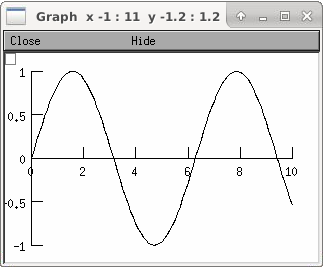
The most basic interpreter prototype for producing a plot follows:
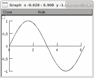
from neuron import h, gui
import math

# Create the graph
g = h.Graph()

# specify coordinate system for the canvas drawing area
# numbers are: xmin, xmax, ymin, ymax respectively
g.size(0, 10, -1, 1)

# the next g.line command will move the drawing pen to the
# indicated point without drawing anything
g.beginline()

# define a sine wave, 0 <= x <= 10
for i in range(101):
    x = i * 0.1
    g.line(x, math.sin(x))

# actually draw the plot on the graph in the window
g.flush()
- Graph.xaxis()
- Syntax:
g.xaxis()g.xaxis(mode)g.xaxis(xstart, xstop)g.xaxis(xstart, xstop, ypos, ntic, nminor, invert, shownumbers)- Description:
The single mode argument draws both x and y axes (no arg == mode 0). See
Graph.yaxis()for a complete description of the arguments.
- Graph.yaxis()
- Syntax:
g.yaxis()g.yaxis(mode)g.yaxis(ystart, ystop)g.yaxis(ystart, ystop, ypos, ntic, nminor, invert, shownumbers)- Description:
The single mode argument draws both x and y axes (no arg == mode 0).
- mode = 0
view axes (axes in each view drawn dynamically) when graph is created these axes are the default
- mode = 1
fixed axes as in long form but start and stop chosen according to first view size.
- mode = 2
view box (box axes drawn dynamically)
- mode = 3
erase axes
- Arguments which specify the numbers on the axis are rounded,
and the number of tic marks is chosen so that axis labels are short numbers (eg. not 3.3333333… or the like).
The xpos argument gives the location of the yaxis on the xaxis (default 0).
- Without the ntic argument (or ntic=-1),
the number of tics will be chosen for you.
- nminor is the number
of minor tic marks.
shownumbers=0 will not draw the axis labels.
invert=1 will invert the axes.
Note:
It is easiest to control the size of the axes and the scale of the graph through the graphical user interface. Normally, when a new graph is declared (eg.
g = h.Graph()), the y axis ranges from 20-180 and the x axis ranges from 50-250. With the mouse arrow on the graph window, click on the right button and set the arrow on View at the top of the button window column. A second button window will appear to the right of the first, and from this button window you can select several options. Two of the most common are:- view=plot
Size the window to best-fit the plot which it contains.
- Zoom in/out
Allows you to click on the left mouse button and perform the following tasks:
- move arrow to the right
scale down the x axis (eg. 50 - 250 becomes 100 - 110)
- “shift” + move arrow to the right
view parts of the axis which are to the left of the original window
- move arrow to the left
scale up the x axis (eg. 50 - 250 becomes -100 - 500)
- “shift” + move arrow to the left
view parts of the axis which are to the right of the original window
- move arrow up
scale down the y axis (eg. 20 - 180 becomes 57.5 - 62)
- “shift” + move arrow up
view parts of the axis which are below the original window
- move arrow down
scale up the y axis (eg. 20 - 180 becomes -10,000 - 5,000)
- “shift” + move arrow down
view parts of the axis which are above the original window
You can also use the size command to determine the size of what you view in the graph window. Eg.
g.size(-1,1,-1,1)makes both axes go from -1 to 1.
- Graph.addvar()
- Syntax:
g.addvar("label", _ref_variable)g.addvar("label", _ref_variable, color_index, brush_index)- Description:
Add the variable to the list of items graphed when
g.plot(x)is called. The address of the variable is used so this is fast. The current color and brush is used if the optional arguments are not present.Additional syntaxes are available for plotting HOC variables.
Note
To automatically plot a variable added to a graph
gwith addvar againsttduring arun(),stdrun.hocmust be loaded (this is done automatically with afrom neuron import gui) and the graph must be added to a graphList, such as by executinggraphList[0].append(g).Example:
g.addvar('Calcium', soma(0.5)._ref_cai)
- Graph.addexpr()
Note
Not that useful in Python; only works with HOC expressions.
- Syntax:
g.addexpr("HOC expression")g.addexpr("HOC expression", color_index, brush_index)g.addexpr("label", "HOC expr", object, ....)- Description:
Add a HOC expression (eg. sin(x), cos(x), exp(x)) to the list of items graphed when
g.plot(x)is called.The current color and brush is used if the optional arguments are not present. A label is also added to the graph that indicates the name of the variable. The expression is interpreted every time
g.plot(x)is called so it is more general thanaddvar(), but slower.If the optional label is present that string will appear as the label instead of the expr string. If the optional object is present the expr will be evaluated in the context of that object.
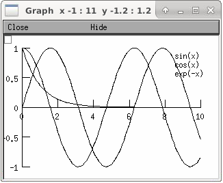
Example:
from neuron import h, gui

g = h.Graph()
g.size(0, 10, -1, 1)
g.addexpr("sin(x)")
g.addexpr("cos(x)")
g.addexpr("exp(-x)")

# have to initialize the variable in HOC
h("x = 0")

g.begin()

for i in range(101):
    h.x = i * 0.1
    g.plot(h.x)

g.flush()
- Graph.addobject()
- Syntax:
g.addobject(rangevarplot)g.addobject(rangevarplot, color, brush)- Description:
Adds the
RangeVarPlotto the list of items to be plotted onGraph.flush()
- Graph.begin()
Note
Not that useful in Python since only works with
Graph.addexpr()which uses HOC expressions.- Syntax:
g.begin()- Description:
Initialize the list of graph variables so the next
g.plot(x)is the first point of each graph line.See
Graph.plot()for an example.
- Graph.plot()
Note
Not that useful in Python since only works with
Graph.addexpr()andGraph.xexpr()which use HOC expressions.- Syntax:
g.plot(x)- Description:
The abscissa value for each item in the list of graph lines. Usually used in a
forloop.See
Graph.plot()for an example.
- Graph.xexpr()
Note
Not that useful in Python since only works with HOC expressions.
- Syntax:
g.xexpr("HOC expression")g.xexpr("HOC expression", usepointer)- Description:
Use this expression for plotting two-dimensional functions such as (x(t), y(t)), where the x and y coordinates are separately dependent on a single variable t. This expression calculates the x value each time
.plotis called, while functions declared by.addexprwill calculate the y value when.plotis called. This can be used for phase plane plots, etc. Note that the normal argument to.plotis ignored when such an expression is invoked. Whenusepointeris 1 the expression must be a variable name and its address is used.
Example:
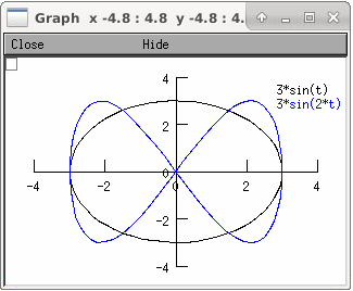
from neuron import h, gui

# Assign "g" the role of pointing to a Graph
# created from the Graph class, and produces
# a graph window with x and y axes on the
# screen.
g = h.Graph()

# size the window to fit the graph
g.size(-4, 4, -4, 4)

# store 3*sin(t) as a function to be plotted in g graphs
g.addexpr('3*sin(t)')

# the next graph will be blue
g.color(3)

# store 3 * sin(2 * t) as a function to be plotted
g.addexpr("3*sin(2*t)")

# store 3*cos(t) as the x function to be plotted in g graphs
# The two previous expressions become the y values
g.xexpr('3*cos(t)')

g.begin()
for i in range(64):
    # h.t ranges from 0 to 6.3 \approx 2 * pi
    h.t = i * 0.1
    g.plot(h.t)

# actually draws the graph
g.flush()
plots a black circle of radius=3 and a blue infinity-like figure, spanning from x=-3 to x=3.
- Graph.flush()
- Syntax:
g.flush()- Description:
Actually draw what has been placed in the graph scene. (If you are continuing to compute you will also need to call
doEvents()before you see the results on the screen.) This redraws all objects in the scene and therefore should not be executed very much during plotting of lines with thousands of points.
Warning
On Microsoft Windows, too many points, too close together will not appear at all on a graph window. You can, in such a case, zoom in to view selected parts of the function.
- Graph.fastflush()
- Syntax:
.fastflush()- Description:
Flushes only the
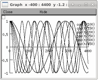
plot()(x) points since the lastflush()(orfastflush). This is useful for seeing the progress ofaddvar()plots during long computations in which the graphlines contain many thousands of points. Make sure you do a normal.flushwhen the lines are complete since fastflush does not notify the system of the true size of the lines. In such cases, zooming, translation, and crosshairs do not always work properly till after theflush()command has been given. (Note, this is most useful for time plots).from neuron import h, gui g = h.Graph() g.size(0, 4000, -1, 1) g.addexpr("cos(t/100)") g.addexpr("cos(t/150)") g.addexpr("cos(t/200)") g.addexpr("cos(t/250)") g.addexpr("cos(t/300)") g.addexpr("cos(t/450)") def pl(): g.erase() g.begin() for h.t in range(4000): g.plot(h.t) if (h.t % 10 == 0) : g.fastflush() h.doNotify() g.flush() h.doNotify() pl()
- Graph.family()
- Syntax:
g.family(boolean)g.family("varname")- Description:
The first form is similar to the Keep Lines item in the graph menu of the graphical user interface.
- 1
equivalent to the sequence —Erase lines; Keep Lines toggled on; use current graph color and brush when plotting the lines.
- 0
Turn off family mode. Original color restored to plot expressions; Keep Lines toggled off.
With a string argument which is a variable name, the string is printed as a label and when keep lines is selected each line is labeled with the value of the variable.
When graphs are printed to a file in Ascii mode, the lines are labeled with these labels. If every line has a label and each line has the same size, then the file is printed in matrix form.
- Graph.vector()
- Syntax:
.vector(n, _ref_x, _ref_y)
Description:
Rudimentary graphing of a y-vector vs. a fixed x-vector. The y-vector is reread on each
.flush()(x-vector is not reread). Cannot save and cannot keep lines.Note
For plotting
Vectorobjects, it is typically easier to useVector.plot(),Vector.line(), andVector.mark().Note
A segmentation violation will result if n is greater than the vector size.
Example:
from neuron import h, gui
import numpy

num_elements = 629

x = h.Vector(num_elements)
y = h.Vector(num_elements)

# fill x with 0, 0.01, 0.02, etc
x.indgen(0.01)

# set y to the sin of x via numpy
y.as_numpy()[:] = numpy.sin(x)

# create the graph
g = h.Graph()
g.size(0, 6.28, -1, 1)
g.vector(num_elements, x._ref_x[0], y._ref_x[0])
g.flush()
- Graph.getline()
- Syntax:
thisindex = g.getline(previndex, xvec, yvec)- Description:
Copy a graph line into the
Vector‘s xvec and yvec. Those vectors are resized to the number of points in the line. Also, if the line has a label, it is copied to the vector as well (seeVector.label()). The index of the line is returned. To re-get the line at a later time (assuming no line has been inserted into the graphlist earlier than its index value — new lines are generally appended to the list but if an earlier line has been removed, the indices of all later lines will be reduced) then use index-1 as the argument. Note that an argument of -1 will always return the first line in the Graph. If the argument is the index of the last line then -1 is returned and xvec and yvec are unchanged. Note that thisindex is not necessarily equal to previndex+1.- Example:
To iterate over all the lines in
h.Graph[0]use:xline = [] yline = [] xvec = h.Vector() yvec = h.Vector() j = 0 i = h.Graph[0].getline(-i, xvec, yvec) while i != -1: # xvec and yvec contain the line with Graph internal index i. # and can be associated with the sequential index j. print(j, i, yvec.label) xline.append(xvec.c()) yline.append(yvec.cl()) # clone label as well i = h.Graph[0].getline(i, xvec, yvec)
- Graph.line_info()
- Syntax:
thisindex = g.line_info(previndex, vector)- Description:
For the next line after the internal index, previndex, copy the label into the
Vectorvectoras well as colorindex, brushindex, label x location, label y location, and label style and return the index of the line. If the argument is the index of the last line then -1 is returned and Vector is unchanged. Note that an argument of -1 will always return the line info for the first polyline in the graph.
- Graph.erase()
- Syntax:
g.erase()- Description:
Erase only the drawings of graph lines.
- Graph.erase_all()
- Syntax:
g.erase_all()- Description:
Erase everything on the graph.
- Graph.size()
- Syntax:
g.size(xstart, xstop, ystart, ystop)g.size(1-4)g.size(_ref_dbl)
Description:
- .size(xstart, xstop, ystart, ystop)
The natural size of the scene in model coordinates. The “Whole Scene” menu item in the graphical user interface will change the view to this size. Default axes are this size.
- .size(1-4)
Returns left, right, bottom or top of first view of the scene. Useful for programming.
- .size(_ref_dbl)
Returns the xmin, xmax, ymin, ymax values of all marks and lines of more than two points in the graph in dbl[0],…, dbl[3] respectively. This allows convenient computation of a view size which will display everything on the graph. See View = Plot. In the absence of any graphics, it gives the size as in the .size(1-4) prototype. (e.g. if
dbl = h.Vector(4), then useg.size(dbl._ref_x[0])to store starting at the beginning.)
- Graph.label()
- Syntax:
.label(x, y, "label").label(x, y).label("label").label(x, y, "string", fixtype, scale, x_align, y_align, color)
Description:
.label(x, y, "label")Draw a label at indicated position with current color.
.label("label")Add a label one line below the previous label
.label(x, y)Next
label("string")will be printed at this location
The many arg form is used by sessions to completely specify an individual label.
- Graph.fixed()
- Syntax:
.fixed(scale)- Description:
Sizes labels. Future labels are by default attached with respect to scene coordinates. The labels maintain their size as the view changes.
- Graph.vfixed()
- Syntax:
.vfixed(scale)- Description:
Sizes labels. Future labels are by default attached with respect to relative view coordinates in which (0,0) is the left,bottom and (1,1) is the right,top of the view. Thus zooming and translation does not affect the placement of the label.
- Graph.relative()
- Syntax:
.relative(scale)- Description:
I never used it so I don’t know if it works. The most useful labels are fixed in that they maintain their size as the view is zoomed.
- Graph.align()
- Syntax:
.align([x_align], [y_align])- Description:
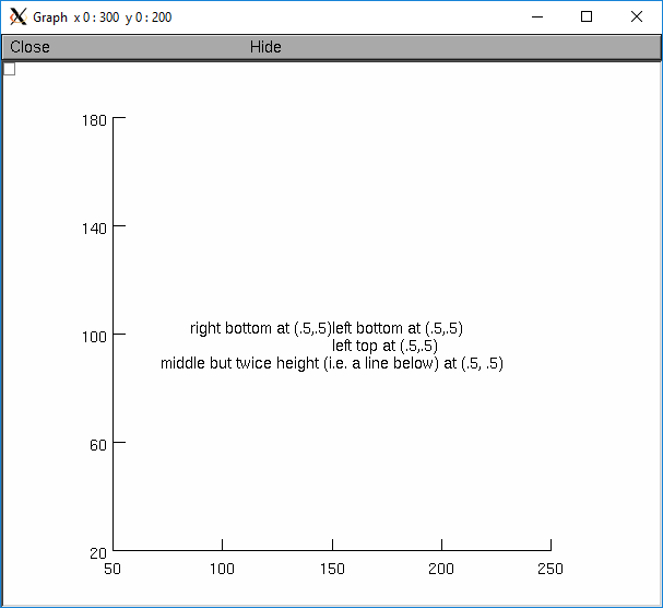
Alignment is a number between 0 and 1 which signifies which location of the label is at the x,y position. .5 means centering. 0 means left(bottom) alignment, 1 means right(top) alignment
Example:
from neuron import h, gui
g = h.Graph()
g.align(0, 0)
g.label(.5,.5, "left bottom at (.5,.5)")
g.align(0, 1)
g.label(.5,.5, "left top at (.5,.5)")
g.align(1, 0)
g.label(.5,.5, "right bottom at (.5,.5)")
g.align(.5,2)
g.label(.5,.5, "middle but twice height (i.e. a line below) at (.5, .5)")
- Graph.color()
- Syntax:
.color(index).color(index, "colorname")- Description:
Set the default color (starts at 1 == black). The default color palette is:
0 white
1 black
2 red
3 blue
4 green
5 orange
6 brown
7 violet
8 yellow
9 gray
.color(index, "colorname")Install a color in the Color Palette to be accessed with that index. The possible indices are 0-100.
The user may also use the colors/brushes button in the graphical user interface, which is called by placing the mouse arrow in the graph window and pressing the right button.
- Graph.brush()
- Syntax:
.brush(index).brush(index, pattern, width)
Description:
.brush(index)Set the default brush. 0 is the thinnest line possible, 1-4 are thickness in pixel. Higher indices cycle through these line thicknesses with different brush patterns.
.brush(index, pattern, width)Install a brush in the Brush Palette to be accessed with the index. The width is in pixel coords (< 1000). The pattern is a 31 bit pattern of 1’s and 0’s which is used to make dash patterns. Fractional widths work with postscript but not idraw. Axes are drawn with the nrn.defaults property
*default_brush: 0.0
The user may also use the ChangeColor-Brush button in the graphical user interface, which is called by placing the mouse arrow in the graph window and pressing the right button.
- Graph.view()
- Syntax:
.view(mleft, mbottom, mwidth, mheight, wleft, wtop, wwidth, wheight).view(2)- Description:
Map a view of the Shape scene. m stands for model coordinates within the window, w stands for screen coordinates for placement and size of the window. The placement of the window with respect to the screen is intended to be precise and is with respect to pixel coordinates where 0,0 is the top left corner of the screen.
The single argument form maps a view in which the aspect ratio between x and y axes is always 1. eg like a shape window.
- Graph.save_name()
- Syntax:
.save_name("objectvar").save_name("objectvar", 1)- Description:
The objectvar used to save the scene when the print window manager is used to save a session. If the second arg is present then info about the graph is immediately saved to the open session file. This is used by objects that create their own graphs but need to save graph information.
- Graph.beginline()
- Syntax:
.beginline().beginline(color_index, brush_index).beginline("label").beginline("label", color, brush)- Description:
State that the next
g.line(x)is the first point of the next line to be graphed. This is a less general command than.begin()which prepares a graph for the.plot()command. The optional label argument labels the line.
- Graph.line()
- Syntax:
.line(x, y)- Description:
Draw a line from the previous point to this point. This command is normally used inside of a
forloop. It is analogous to.plot()and the commands which go along with it but avoids the need to use HOC expressions, since it plots one line at a time.This command takes arguments for both x and y values, so it can serve the same purpose of the
.plotcommand in conjunction with an.addexpr()command and an.xexpr()command.
Example:
from neuron import h, gui
import math

g = h.Graph()
g.size(-1, 1, -1, 1)

g.beginline()
t = i = 0
dt = 0.1
while t <= 2 * math.pi + dt:
    t = i * dt
    g.line(math.sin(t), math.cos(t))
    i += 1

g.flush()
graphs a circle of radius = 1.
- Graph.mark()
- Syntax:
.mark(x, y).mark(x, y, "style").mark(x, y, "style", size).mark(x, y, "style", size, color, brush)- Description:
Make a mark centered at the indicated position which does not change size when window is zoomed or resized. The style is a single character
+, o, s, t, O, S, T, |, -whereo,t,sstand for circle, triangle, square and capitalized means filled. Default size is 12 points. For the style, an integer index, 0-8, relative to the above list may also be used.
- Graph.crosshair_action()
- Syntax:
.crosshair_action(py_callable).crosshair_action(py_callable, vectorflag=0).crosshair_action("")- Description:
While the crosshair is visible (left mouse button pressed) one can type any key and the procedure will be executed with three arguments added:
py_callable(x, y, c)where x and y are the coordinates of the crosshair (in model coordinates) and c is the ascii code for the key pressed.When the optional vectorflag argument is 1, then, just prior to each call of the procedure_name due to a keypress, two temporary
Vectorobjects are created and the line coordinate data is copied to those Vectors. With this form the call to the procedure has two args added:procedure_name(i, c, xvec, yvec)whereiis the index of the crosshair into the Vector.If you wish the Vector data to persist then you can assign to another objectvar before returning from the
py_callable. Note that one can copy any line to a Vector with this method whereas the interpreter controlledGraph.dump("expr", y_objectref)is limited to the current graphline of anaddvaroraddexpr.With an empty string arg, the existing action is removed.
Example:
from neuron import h, gui

g = h.Graph()

def crossact(x, y, c):
  '''For g.crosshair_action(crossact)'''
  print ("x=%g y=%g c=%c" % (x, y, int(c)))

def crossact_vflag1(i, c, xvec, yvec):
  '''For g.crosshair_action(crossact_vflag1, 1)'''
  i = int(i)
  print ("i=%d x[i]=%g y[i]=%g c=%c" % (i, xvec[i], yvec[i], int(c)))

g.crosshair_action(crossact_vflag1, 1)

# plot something
x = h.Vector().indgen(50, 100, 1)
y = x + 50 # needs NEURON 7.7+
y.line(g, x)

# now click/drag on the plotted line and occasionally press a key
Example:
from neuron import h, gui
import numpy

num_elements = 629

x = h.Vector(num_elements)
y = h.Vector(num_elements)

# fill x with 0, 0.01, 0.02, etc
x.indgen(0.01)

# set y to the sin of x via numpy
y.as_numpy()[:] = numpy.sin(x)

# create the graph
g = h.Graph()
g.size(0, 6.28, -1, 1)
g.vector(num_elements, x._ref_x[0], y._ref_x[0])

def crosshair(x, y, key):
    print('x = %g, y = %g, key = %c' % (x, y, key)(

g.crosshair_action(crosshair)

g.flush()
To test the crosshair_action functionality, run the above code, move the mouse over the graph with the left mouse button held down, and simultaneously press a key; the coordinates and the key pressed will be displayed in the terminal.
Note
Python support for
Graph.crosshair_actionwas added in NEURON 7.5.See also
- Graph.view_count()
- Syntax:
.view_count()- Description:
Returns number of views into this scene. (stdrun.hoc removes scenes from the
flush_listandgraphList[]when this goes to 0. If no otherobjectvarpoints to the scene, it will be freed.)
- Graph.unmap()
- Syntax:
.unmap()- Description:
Dismiss all windows that are a direct view into this scene. (does not unmap boxes containing scenes.)
.unmapis called automatically when no hoc object variable references the Graph.
- Graph.printfile()
- Syntax:
.printfile("filename")- Description:
Print the first view of the graph as an encapsulated post script file.
- Syntax:
g.menu_remove("item name")- Description:
Removes the named menu item from the Graph instance.
- Syntax:
g.exec_menu("item name")- Description:
Equivalent to by pressing and releasing one of the items in the Graph menu with the right mouse button. This executes an action for regular items, toggles for items like “Keep Lines”, and specifies the left mouse tool for radio buttons. The “item name” must be identical to the string in the menu item, including spaces and case. Some items may not work unless the graph is mapped to the screen. Selection is with respect to the primary (first) view, eg selecting “View = plot” of a Grapher will always refer to the view in the Grapher tool as opposed to other views of the same graph created via the “NewView” menu item. Any items created with
Graph.menu_action()orGraph.menu_tool()are selectable with this function.
Example:
g = h.Graph()
g.exec_menu("Keep Lines")
- Syntax:
.menu_action("label", py_callable)- Description:
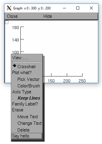
Add a menu item to the Graph popup menu. When pressed, the py_callable will be called.
Example:
from neuron import h, gui

def say_hi():
    print('Hello world!')

g = h.Graph()
g.menu_action("Say hello", say_hi)
- Syntax:
.menu_tool("label", "procedure_name").menu_tool("label", "procedure_name", "select_action")- Description:
Add a selectable tool menu item to the Graph popup menu or else, if an
xpanel()is open, anxradiobutton()will be added to the panel having the same action. (note: all menu_tool radiobuttons whether in the graph menu or in a panel, are in the same telltalegroup, so selecting one deselects the previous selection.)If the third arg exists, the select_action will be executed when the radioitem is pressed (if it is not already selected).
When selected, the item will be marked and the label will appear on the window title bar (but not if the Graph is enclosed in a
VBox()). When this tool is selected, pressing the left mouse button, dragging the mouse, and releasing the left button, will cause procedure_name to be called with four arguments: type, x, y, keystate. x and y are the scene (model) coordinates of the mouse pointer, and type is 2 for press, 1 for dragging, and 3 for release. Keystate reflects the state of control (bit 1), shift (bit 2), and meta (bit 3) keys, ie control and shift down has a value of 3.The rate of calls for dragging is of course dependent on the time it takes to execute the procedure name.
Example:
from neuron import h, gui

def on_event(event_type, x, y, keystate):
    print(event_type, x, y, keystate)

g = h.Graph()
g.menu_tool("mouse events", on_event)
In this example, you must first select “mouse events” from the Graph’s menu, then left-click or drag over the graph, optionally while holding a modifier key; output will appear on the terminal.
- Graph.gif()
- Syntax:
g.gif("file.gif")g.gif("file.gif", left, bottom, width, height)- Description:
Display the gif image in model coordinates with lower left corner at 0,0 or indicated left, bottom coords. The width and height of the gif file are the desired width and height of the image in model coordinates, by default they are the pixel Width and Height of the gif file.
- Example:
Suppose we have a gif with pixel width and height, wg and hg respectively. Also suppose we want the gif pixel point (xg0, yg0) mapped to graph model coordinate (x0, y0) and the gif pixel point (xg1, yg1) mapped to graph model coordinate (x1, y1). Then the last four arguments to g.gif should be:
left = x0 - xg0*(x1-x0)/(xg1-xg0)
bottom = y0 - yg0*(y1-y0)/(yg1-yg0)
width = wg*(x1-x0)/(xg1-xg0)
height= hg*(y1-y0)/(yg1-yg0)
If, for example with xv, you have constructed a desired rectangle on the gif and the info (xv controls/Windows/Image Info)presented is Resolution: 377x420 Selection: 225x279 rectangle starting at 135,44 then use
{wg=377 hg=420}
{xg0=135 yg0=420-(279+44) xg1=135+225 yg1=420-44}
Warning
In the single arg form, if the gif size is larger than the graph model coodinates, the graph is resized to the size of the gif. This prevents excessive use of memory and computation time when the graph size is on the order of a gif pixel.
- Graph.view_info()
- Syntax:
i = g.view_info()val = g.view_info(i, case)val = g.view_info(i, case, model_coord)
Description:
Return information about the ith view.
With no args the return value is the view number where the mouse is. If the mouse was not last in a view of g, the return value is -1. Therefore this no arg function call should only be made on a mouse down event and saved for handling the other mouse events. Note that the two arg cases are generally constant between a mouse down and up event.
    case 1: // width
    case 2: // height
    case 3: // point width
    case 4: // point height
    case 5: // left
    case 6: // right
    case 7: // bottom
    case 8: // top
    case 9: // model x distance for one point
    case 10: // model y distance for one point
The following cases (11 - 14) require a third argument
relative location means (0,0) is lower left and (1,1) is upper right.
    case 11: // relative x location (from x model coord)
    case 12: // relative y location (from y model coord)
    case 13: // points from left (from x model coord)
    case 14: // points from top (from y model coord)
            Note: this last is from the top, not from the bottom.
    case 15: // height of font in points
- Graph.view_size()
- Syntax:
g.view_size(i, left, right, bottom, top)- Description:
Specifies the model coordinates of the ith view of a Graph. It is possible to use this in a
Graph.menu_tool()callback procedure.
- Graph.glyph()
- Syntax:
g.glyph(glyphobject, x, y, scalex, scaley, angle, fixtype)- Description:
Add the
Glyph()object to the graph at indicated coordinates (the origin of the Glyph will appear at x,y) first scaling the Glyph and then rotating by the indicated angle in degrees. The last four arguments are optional and have defaults of 1,1,0,0 respectively. Fixtype refers to whether the glyph moves and scales with zooming and translation, moves only with translation but does not scale, or neither moves nor scales.
- Graph.simgraph()
- Syntax:
g.simgraph()- Description:
Adds all the
Graph.addvar()lines to a list managed byCVodewhich allows the local variable time step method to properly graph the lines. See the implementation in share/lib/hoc/stdrun.hoc for usage.